
ADVERTISEMENTS:
Having studied a producer’s behaviour in short run with the help of a production function with one variable input (viz. labour), holding other factors constant, we now focus on the same in long run in which all factors of production are variable. It means that in a two factor model a firm can vary both labour and capital to increase production in long run.
The basic objective of a producer is to find out an optimum combination of the two factors from among the available ones which leads to a minimum cost for a specified level of output or maximum output from a given stock of inputs. It will enrich our knowledge with regard to returns to scale originating from scale economies.
Production Function in Long Run:
Given that a firm can make all kinds of adjustments in its production process in long run, its production function can be written as,
ADVERTISEMENTS:
Q = f (L, K)
It is also called as production with two variable factor inputs, labour (L) and capital (K) in particular. A commonly discussed form of long run production function is the Cobb-Douglas production function which is an example of linear homogenous production functions.
Linear Homogenous Production Functions:
Basic features of such a production function can be explained in terms of its two components — (i) linear function and, (ii) homogeneity of function.
The linear production functions are the fixed proportion production functions represented by a straight line expansion path, which passes through the point of origin. They are also known as Leontief Production Function as they were first evolved by Prof. Leontief.
ADVERTISEMENTS:
Such a production function will be homogeneous of degree one when the proportionate change in output is same as the proportionate change in the inputs implying a constant return to scale.
To show this, let us consider a general production function —
Q = f (L, K)
Now, both the factors of production are increased by a proportion λ (Lambda) resulting into a higher output represented by Q*. Hence, the function can be written as —
ADVERTISEMENTS:
Q* = f (λL, λK)
If λ can be taken out as a common factor, than the increased new level of output will be initial output multiplied by λ powered by ʋ (Greek letter Upsilon)

If the ʋ is equal to 1 then the production function will be a homogenous of degree one representing constant returns to scale. But, if the ʋ is not equal to 1 then the production function will be non-homogenous representing increasing (ʋ > 1) or diminishing (ʋ < 1) return to scale.
ADVERTISEMENTS:
In short, the production function will represent:
i. Constant returns to scale when ʋ = 1; homogenous production function
ii. Increasing returns to scale when ʋ > 1; non homogenous production function
iii. Decreasing returns to scale when ʋ < 1; non homogenous production function
Cobb-Douglas Production Function:
ADVERTISEMENTS:
A very common form of linear homogenous production functions is the Cobb-Douglas production function which is based on empirical evidences mainly from US industry data. It was first developed in 1927 and represented as —

Here Q is a dependent variable representing output level and, L and K denotes labour and capital respectively. The A, α and β are positive co-efficient.
i. The coefficient A is relates to technology and represents the efficiency level in the production. Higher the value of A, more advanced will be technology.
ii. The coefficient α denotes labour productivity, i.e., the contribution of labour in the production function. Technically, it measures a percentage increase in output as a result of a one per cent increase in labour input while K remaining same. For example, if α = 0.20, a one percentage increase in labour would lead to a 0.2 per cent increase in output.
iii. In a similar fashion, the β shows capital productivity and measures a percentage increase in output associated with a one per cent increase in capital input while L remaining same.
iv. Both the α and β are also termed as output elasticity of labour and capital respectively.
The Cobb-Douglas production function can be applied to derive laws of returns to scale, as per the following schedule:

When α + β = 1, than β can be written as 1 – α and, the Cobb-Douglas the production function as —
Q = A.LαK1–α
Such a form of production function will be called as homogenous of degree one when α + β = 1.
The marginal product and average product of the two factors in a Cobb- Douglas production function will depend upon the factor ratio, i.e. (K/L).
In other words, absolute volume of labour and capital used in the production will have no impact on average and marginal factor products so far the K/L remains the same.
The empirical evidences gathered from the US manufacturing industries, as published in American Economic Review 1948, showed that in most industries constant returns to scale has prevailed. Thus, the production processes are well described by a linear homogeneous function with an elasticity of substitution of one between factors.
It is indicated that capital contribution in production in US industries was around 75% while rest (25%) by labour. It was subsequently confirmed by the National Bureau of Economic Research.
Producer’s Behaviour:
To study a producer’s behaviour when both the factors of production are variable under the two factor framework, we need to develop a new tool of analysis which is named as isoquant. It is conceptually similar to the indifference curve of the consumer theory.
Needless to add, basic framework and properties of an isoquant will be broadly similar to that of an indifference curve. The isoquant analysis will enable us to find out not only the producer’s equilibrium in the long run but will also help us to study returns to scale graphically.
Equilibrium of a Producer:
The producer being rational will find his equilibrium when:
1. Cost minimizes for a given output level or, cost minimization subject to an output constraint or,
2. Output maximizes from a given total outlay or output maximization subject to a cost constraint.
Assumptions of a Producer’s Equilibrium:
1. The producer is rational i.e. he aims to maximize profits.
2. Producer employs only two factors of production. All units of each factor are homogeneous.
3. The factor-prices are given and constant.
4. There is a perfect competition in factor market.
Conditions of Equilibrium:
Producer’s equilibrium is subject to satisfaction of following two conditions:
1. Slope of isoquant should be equal to slope of iso-cost line. i.e.
MRTSLK = MPL/MPK = w/r = PL/PR
Or, MPL/MPK = w/r
This will happen when the iso-cost line forms a tangent on a point on the isoquant. It is called as the first order condition or necessary condition.
2. At the point of equilibrium, the isoquant should be convex to the origin. This is known as sufficient condition.
Minimizing Cost Subject to an Output Constraint:
This is a case in which a producer attempts to find out a minimum cost of producing a certain amount of output.
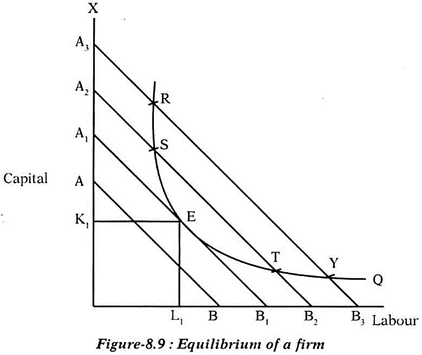
Such a case has been presented in Figure-8.9 and has been discussed below:
i. As the output level is given (i.e. an output constraint), there will only be one isoquant (Q) representing the desired level of output.
ii. Against it, the firm will have a couple of parallel iso-cost lines, AB, A1B1, A2B2 and, A3B3 in the figure, representing different levels of total outlay. More the distance of a line from the point of origin higher will be the total outlay. Thus, line AB represents a least total outlay while A3B3 highest total outlay level. All of them have same slope since factor price ratio (w/r) is same on all of them.
iii. The iso-cost line AB does not come in contact with the isoquant at any of its point and hence cannot produce the Q level of output.
iv. Remaining three iso-cost lines, however, meet the isoquant at different points (R, S, E, T and V) and, hence, has to be considered by the producer. All of them provide viable solutions to the producer.
v. However, since the objective is to produce the Q level of output at a minimum cost, the producer will reject all the options except E which lies on A1B1. All the rejected options lie on the iso-cost lines which are at a distance more than A1B1 from the point of origin. They, therefore, represent higher outlays.
vi. At point E, both the equilibrium conditions are satisfied – iso-cost line A1B1 is tangent to the isoquant Q and the isoquant is convex to the origin. This shows that the point E (OL1 + OK1) represents a minimum cost for producing Q level of output.
Maximizing Output Subject to a Cost Constraint:
The second case of a producer’s equilibrium is related to a cost constraint for a maximum output of a product.
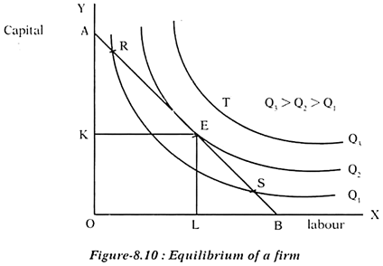
This has been presented in Figure-8.10 and has been discussed below:
i. The total outlay being given, there will be a single iso-cost line, AB, at the given factor prices. The producer will target at a maximum output from it.
ii. For this purpose, an isoquant map consisting of three isoquants Q1 to Q3, indicating different output levels, is drawn.
iii. Point T lies on the highest isoquant (Q3) and, hence, represents a maximum output but it is out of the producer’s reach due to cost constraint, AB. Hence, it has to be ruled out.
iv. The iso-cost line comes in contact with the isoquants at three points, R, E and S. While R and S lie on a lower isoquant (Q1), E lies on a higher one (Q2). Thus, the producer will reject points R and S for point E.
v. Further, the point E satisfies both the conditions of equilibrium – the iso-cost line AB is tangent to the isoquant Q2 at point E and the isoquant Q2 is convex to the origin.
vi. Hence, the producer will be in equilibrium at point E producing Q2 level of output which is the maximum he can produce from the given outlay and factor prices. He will employ OL of labour and OK of capital.
Expansion Path:
Expansion path may be defined as the locus of points which show all the least cost combinations of factors corresponding to different levels of output. In other words, an expansion path traces the movement of the producer from one optimum combination of inputs to another, as there is a change either in his total outlay or in the factor prices.
In simple words, a producer will produce any level of output on the expansion path in such a way that both the conditions of equilibrium are satisfied. A line or curve representing all such combinations of inputs for different levels of output is known as expansion path.
One way of deriving a long run expansion path involves a change in outlay of the firm while keeping the factor prices same. As a result, the iso-cost line will shift in a parallel fashion upward (when total outlay increases) or downward (when it declines). At each outlay level, firm will find its equilibrium subject to satisfying both equilibrium conditions. As the outlay increases, the equilibrium level of output will also increase.
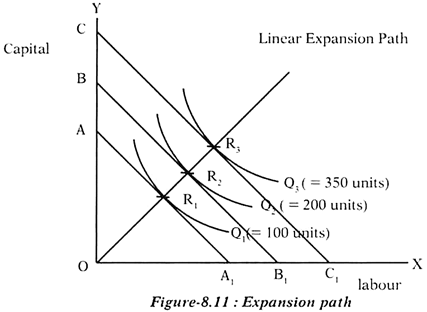
This is shown in Figure-8.11 and discussed below:
i. In the figure, three levels of outlay are represented by three parallel iso-cost lines AA1, BB1 and CC1. They, however, represent a same slope as the factor prices are same for each of them. Each iso-cost line will show an equilibrium level of output.
ii. It is Q1 (=100 units) when total outlay is represented by the iso-cost line AA1, Q2 (=200 units) by the line BB1 and, Q3 (=300 units) by CC1. The respective points of equilibrium or optimal combination are R1, R2, and R3 where both equilibrium conditions are satisfied.
iii. The line joining all the points of equilibrium is known as the expansion path.
The expansion path so derived shows that in order to produce higher levels of output the firm will use increased quantities of both the factors i.e., the scale of production will undergo a change. Hence the expansion path is also known as the scale line. Based on this, the laws of returns to scale can be explained.
Comments are closed.