
ADVERTISEMENTS:
The market price of a commodity is determined by demand and supply. The market has two sides — buyers and sellers. In a typical market there are a number of consumers of a good. We can add up their individual demand curves to arrive at the market demand curve.
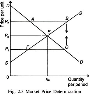
Similarly by adding up the supply curves of independent producers of the good, we arrive at the market supply curve. In Fig. 2.3 two curves meet at point E and the equilibrium price P0 is determined by the impersonal market forces of demand and supply.
The equilibrium price of a good is the price at which the supply of the good equals the demand. The individual buyers and sellers are assumed to take prices as given —outside of their control — and simply determine their optimal response given those market prices A market where each economic agent takes the price as beyond his control is called a competitive market.
ADVERTISEMENTS:
This assumption is justified on the ground that each consumer or producer is a small part of the market as a whole and thus has hardly any influence on the market price by buying or selling a little more or less of the commodity For example, each supplier of wheat takes the market price to be outside his own control.
So he has to decide how much wheat to produce and supply to the market. At the same time the market price itself is determined by the actions of all the agents taken together. Although the market price is independent of any one agent’s actions in a competitive environment if aggregate supply increases price will fall and if aggregate demand increases price will rise.
If D(p) is market demand function and S(p) is the market supply function then the equilibrium price (p0) is the one at which:
ADVERTISEMENTS:
D (p0) = S(p0) .. (1)
Only at a particular price, viz., the equilibrium price, market demand equals market supply In other words, as per the solution to equation (1), p0 is the price where market demand equals market supply. At any other price (called disequilibrium price) there will either occur excess demand or excess supply because the behaviour of different economic agents will not be consistent with one another.
At a disequilibrium price, the behaviours of some buyers and/or sellers would be infeasible. So there would be a reason for their behaviour to change. This means that a disequilibrium price cannot be expected to persist since at least some buyers or sellers would have a tendency to change their behaviour.
The demand and supply curves show the optimal choices of buyer (demanders) and sellers (suppliers). Secondly the fact that they are the same at the equilibrium price p0 simply suggest that their behaviours are compatible. At a disequilibrium price these two conditions will not be met.
ADVERTISEMENTS:
For example at price p1 < p0, there is excess demand (shortage). This means that some suppliers will be able to charge higher prices from the disappointed demanders. As the quantity offered for sale increases, the market price will be pushed up to the equilibrium level at which D(p0) = S(p0).
On the other hand if actual price goes above the equilibrium level (p2 > P0) there will excess supply (surplus). Then some suppliers will be left with unsold stocks. So they will offer their output at a lower price to clear their stocks. But if some suppliers reduce their prices, others who sell identical goods will be forced to make matching price cuts in order to remain competitive.
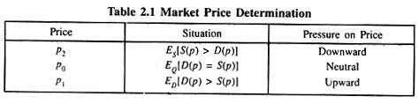
Thus excess supply exerts a downward pressure on the equilibrium price p0. Only when the amount that consumers want to buy at a given price equals the amount that producers want to sell at that price will the market be in equilibrium. See Table 2.1 which summarizes possible market movements.
Two Special Cases:
In case of fixed supply, equilibrium quantity is determined entirely by the supply conditions and the equilibrium price by demand conditions. As shown in Fig. 2.4(a), if the supply curve is vertical the equilibrium price is determined solely by the demand curve. Such a supply curve is said to be completely price inelastic.

In Fig 2.4 (b), where the supply curve is a horizontal straight line, the equilibrium price is determined entirely by the supply curve while the equilibrium quantity is determined by the demand curve. In these, two special cases we have separated the determination of equilibrium price and quantity.
But in the general case equilibrium price and equilibrium quantity are simultaneously determined by the demand and supply curves.
Inverse Demand and Supply Curves:
Individual demand curves normally indicate the optimal quantity demanded as a function of the price charged. But we can also look at them as inverse demand functions. Such demand functions measure the price that someone is ready to pay in order to acquire a certain specific quantity of a good.
ADVERTISEMENTS:
Again normal supply functions measure the quantity supplied of a commodity as a function of its price. Alternatively inverse supply functions measure the price that must prevail in order to ensure that a certain fixed amount of a commodity is offered for sale in the market place.
If we generalize and construct market demand and market supply curves, we can show that the equilibrium price is determined by finding that quantity the demanders are willing to consume is the same as the price that suppliers must receive in order to offer that quantity for sale.
Thus in equilibrium we have:
Ps(q0) = Pd(q0)
where Ps(q0) and Pd(q0) are the inverse supply and demand functions, respectively.
Equilibrium with Linear Demand Curves:
Let us suppose both the demand and supply curves are linear:
D(p) = a – bp …… (2)
S(p) = c + dp ……(3)
The coefficients a and c are intercept parameters and b and d are slope parameters.
The equilibrium price can be found by solving the following equation:
a – bp = c + dp …… (4)
Since, in equilibrium, D(p) = S(p).
From equation (4) we get;
p0 = a – c/a + b
The equilibrium quantity demanded (and supplied) is;
D(p0) = a – bp0
= a – b a – c/d + b = ad + bc/b + d …. (5)
The same result can be obtained by using the inverse demand and supply curves. The equation of the inverse demand curve is;
q = a – bp …… (6)
which indicates at what price is some quantity q demanded. Equation (6) is obtained by substituting q for D(p) and solving for p. From equation (6) we get;
Pd(q) = a – q/b
In the same way we get the equation of the inverse supply curve;
Ps(q) = q – c/d
Equating the demand price with the supply price and solving for the equilibrium quantity we get;
Pd(q) = a – q/b = q – c/d = Ps(q)
Or q0 = ad + bc/b + d ……….. (7)
This equation gives the same values for both the equilibrium price and the equilibrium quantity as equation (5).
Example:
Suppose that the demand function of wheat is Qd = 3550 – 260P and supply function of wheat Qs = 1800 + 240P where P = price in Rs. per quintal of wheat, Qd = quantity of wheat (in quintals) demanded and Qs = quantity of wheat (in quintals) supplied. Determine equilibrium price and quantity of wheat.
Solution:
In equilibrium Qs = Qd or 1800 + 240P = 3550 – 260P, or 500P = 1750
or, P = 3.5 and Qs = Qd = 2640.
Impact of Changes in Demand and Supply:
An equilibrium is found by equating demand with supply (or the demand price with the supply price). Now the equilibrium price will change if the demand and supply curves change, (i.e., shift to a new position). See Fig. 2.5. If the demand curve shifts to the right, then equilibrium price and quantity will both rise (compare points E and F).
Thus when the demand curve shifts the price and quantity move in the same direction and when the supply curve shifts price and quantity move in the opposite direction.
If both the curves shift to the right, equilibrium quantity will surely rise, but price may rise, fall or remain unchanged (compare points E and H). In case of parallel rightward shift of both the curves, the quantity supplied increases by the same fixed amount, say m, at every price. So the new equilibrium condition is;
D(p) + m = S(p) + m
which has the same solution as the original demand equals supply condition.
Comments are closed.