
ADVERTISEMENTS:
The focus will now be on general shapes of indifference curves. To start with we make some general assumptions about preferences and then explore the implications of these assumptions for the shapes of the associated indifference curves.
These assumptions are the defining features for well-behaved (normal) indifference curves.
1. Monotonicity of Preferences:
First we talk about goods not bads. This means that more of a good is always better than less of it. To be more specific, if (x1, x2) is a bundle of goods and (y1, y2) is another bundle with at least as much of one good and more of another, then (y1,y2) > (x1,x2).
ADVERTISEMENTS:
This assumption is known as monotonicity of preferences. The assumption of satiation, i.e., ‘more is better than less’ would probably hold up to a point. The monotonicity assumption suggests that in a world of scarcity we are going to examine situations before the satiation point is reached — while more is still better.
Implications for Indifference Curves:
The monotonicity assumption implies that indifference curves have a negative slope. For example, in Fig. 4.11 a movement anywhere up and to the right from an initial bundle (x1, x2) implies a preferred position. It is because any point to the right of (x1, x2) represents a higher indifference curve which indicates a preferred combinations of the two commodities.
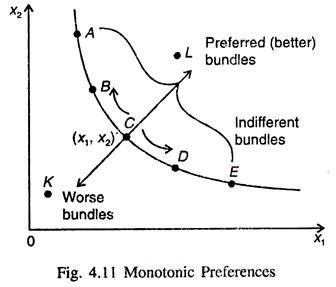
The converse is also true. Any movement down and to the left implies a movement to a worse position. So it logically follows that if a consumer is moving to an indifferent position he must be moving either left and up from point C to B or right and down from C to D : the indifference curve must have a negative slope.
ADVERTISEMENTS:
In short, monotonic preference implies that more of the both goods is a better bundle for this consumer; less of both goods represent a worse bundle. Compare point C with points K and L.
2. Preference for Averages (Means), Rather than Extremes:
The second important assumption about well-behaved indifference curves is that averages are preferred to extremes.
This means that if we consider two bundles of goods (x1, x2) and (y1, y2) or the same indifference curve and take a weighted average of the two bundles such as:
ADVERTISEMENTS:
(1/2 x1 + 1/2y1, ½ x2 + 1/2y2)
then the average bundle will be strictly preferred to each of the two extreme bundles. This weighted-average bundle consists of the average amount of good 1 and the average amount of good 2 that is present in two the bundles (x1, x,) and (y1, y2). So it must lie at the midpoint of straight a line that connects the two bundles.
In a more general situation for any weight k (lying between 0 and 1) and not just 1/2, we are assuming that if (x1, x2) ~ (y1, y2) then:
[kx1 + (1 – k)y1, kx2 + (1 – k)y2] > (x1, x2).
ADVERTISEMENTS:
This weighted-average of the two bundles gives a weight of k to the x-bundle and a weight 1 – k to the y bundle. This means that the distance from the X-bundle to the average bundle is a proportion of k of the distance from the X-bundle to the F-bundle, along the straight line which connects the two bundles (x1, x2) and (y1, y2).
The Concept of ‘Convex Set’:
The above assumption about preference implies that the set of bundles weakly preferred to (x1, x2) is a convex set. Let us suppose (y1, y2) and (x1, x2) are indifferent bundles. Therefore, if averages are preferred to extremes, all of the weighted averages of (x1, x2) and (y1, y2) are weakly preferred to (x1, x2) and (y1, y2).
According to Nobel Laureate economist T. C. Koopmans (c.f., Three Essays on the State of Economic Science) a convex set has the property that if we take any two points in the set and draw a line segment connecting them, then the line segment will lie entirely on the set.
ADVERTISEMENTS:
Fig. 4.12(a) illustrates the concept of convex set, while Fig 4.12(b) and 4.12(c) illustrate two situations involving non-convex preferences. Fig 4.12(c) presents a non-convex set that is called ‘concave preference’.
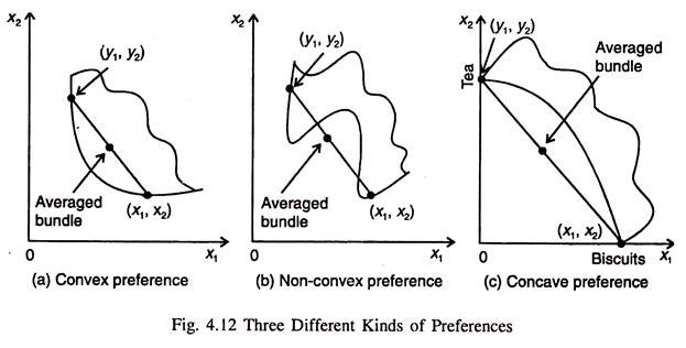
An Example of Non-Convex Preferences: Case of Tea and Biscuits:
In this context we can give an example of non-convex preference. A consumer may like both tea and biscuits. But he does not like to have them together. In considering his consumption in the next three hours he might be indifferent between consuming 2 cups of tea and 4 biscuits, or 4 cups of tea and 2 biscuits.
But either of these bundles would be better than consuming 3 cups of tea and 3 biscuits. This type of preference is shown in the Fig. 4.12(c).
The Rationale behind Convex Preferences:
Well-behaved preferences are convex because, for the most part, goods are consumed together. The kinds of preferences shown in Fig. 4.12(b) and Fig. 4.12(c) imply that the consumer would prefer to specialise in consumption, at least to some extent, and to consume only one of the two goods. Such a situation is known as monomania.
‘Mono’ means one and ‘mania’ means lust (passionate desire) such as the mercantilists’ strong liking for gold. But these are exceptions rather than rules. In most normal situations the consumer would want to trade some of one good for the other and end up consuming some of each, rather than specialising in the consumption of only one of the two goods.
In truth, if an average consumer looks at his preference closely for weakly (monthly) consumption of tea and biscuits rather than his immediate (hourly) consumption he would tend to look much like Fig 4.12(a) rather than Fig. 4.12(c).
Each month he would prefer to have some tea and some biscuits — not necessarily at the same time — rather than specialise in consuming either one for the whole month. Thus time plays an important role in determining a consumer’s preferences.
Comments are closed.