
ADVERTISEMENTS:
Here is a list of examples of consumer preferences.
1. Perfect Substitutes:
Two goods are perfect substitutes if the consumer is ready to substitute one for the other at a constant rate, or, to be more specific, if the consumer is willing to substitute the goods on a one-to-one basis.
Suppose a consumer uses both blue pencil and black pencil without being bothered about colour at all. Let him choose a consumption bundle (5, 5). Then another consumption bundle which contains 10 pencils of the same colour (either blue or black) in it is equally preferable. This means that any consumption bundle (x1, x2) such that x1 + x2 = 20 will lie on this consumer’s indifference curve through (10, 10). In this case the indifference curves will be parallel straight lines with a slope of -1 as shown in the Fig. 4.5.

If the original bundle consists of 5 pencils of each colour and the consumer uses one more blue pencil, then he can use one less black pencil, i.e., 4 to get back to the original indifference curve. Thus the indifference curve through (5, 5) has a slope of -1. This statement is true in case of any bundle of goods with the result that all the indifference curves have a constant slope of -1.
If we show blue pencils on the vertical axis and pairs of black pencils on the horizontal axis the indifference curves would have a slope of -2. It is because the consumer would be willing to sacrifice one blue pencil to get another pair of black pencils.
2. Perfect Complements:
Perfect complements are goods which are always consumed together as also in a certain fixed proportion. A commonly cited example is left shoes and right shoes which ‘complement’ each other. The consumer wears both shoes together. Having only one out of a pair of shoes serves no purpose.
Suppose a consumer chooses the consumption bundle (3, 3). Now if he is given one more right shoe, he will have (4, 3). This makes the consumer indifferent to the original bundle. The extra shoe is of no use to him. The same thing happens if the consumer is given another left shoe- he is indifferent between (4, 3) and (3, 3).
ADVERTISEMENTS:
In this case the indifferent curves are L-shaped, with the vertex occurring at the elbow of each indifference curve (such as A, B and C) where the number of left shoes equals the number of right shoes as shown in Fig. 4.6.
In case of perfect complements the consumer always wants to consume the goods in fixed proportions to each other. However, that proportion is not always one-to-one. This is why indifference curves are L-shaped with MRS = 0 on the horizontal stretch and MRS → ∝ on the vertical stretch.
If the number of both left shoes and right shoes is increased at the same rate, their proportion remains the same, but the consumer moves to a higher indifference curve, i.e., to a more preferred position.
3. Economic Bads:
ADVERTISEMENTS:
A bad is a commodity that the consumer does not want to consume or even if he consumes it he does not like it at all. For example, suppose that the consumer loves mango but dislikes jackfruit. But we assume that there is no trade-off between the two. That is, there would be some amount of mango in fruit salad that would compensate the consumer for having to consume a given amount of jackfruit.
The indifference curves for a bad are presented in Fig. 4.7. Suppose we give the consumer a bundle (x1, x2) of mango and jackfruit. If we give him some jackfruit we have to give him some mango as compensation. The mango will compensate him for having forced to consume jackfruit which he dislikes and does not want to consume in normal circumstances.
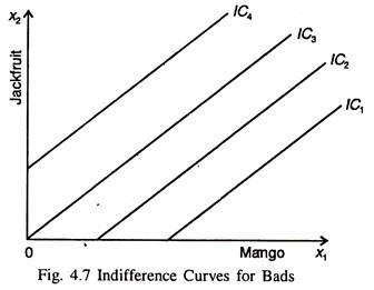
The direction of increased preference is towards decreased jackfruit consumption and increased mango consumption as is indicated by the arrows. Thus indifference curves slope upward and to the right in this case.
4. Neutral Goods:
ADVERTISEMENTS:
If the consumer is not bothered about the consumption of a commodity it is called a neutral good, such as jackfruit (or even guava). If a consumer is just neutral about guava, his indifference curves will be vertical lines as shown in Fig. 4.8.
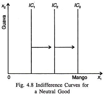
In this case the consumer is bothered about only the number of mangoes he has and does not care at all about how many guavas he has. As the number of mangoes in his possession increases, he feels better and better. But an increase in the consumption of guava does not affect him in any way, i.e., does not make him feel better.
5. Satiation:
One of the assumptions of the theory of consumer behaviour is non-saturation. We assume that the consumer never reaches the saturation point regarding the consumption of a commodity. But sometimes counter examples appear to be interesting. That is why we may consider a situation involving satiation, where there is some overall best bundle for the consumer.
ADVERTISEMENTS:
The closer the consumer is to the best bundle, the better he is in terms of his welfare (preferences). For example, let us suppose that the consumer has some most preferred bundle of goods (x1, x2) as shown in Fig. 4.9.
The farther away he is from that bundle, the worse- off he is in terms of preferences. In this case point B corresponding to the consumption bundle (x1, x2) is a bliss (best) point. And indifference curves such IC1, IC2 and IC3 surround this point. Points farther away from the bliss point lie on ‘lower’ indifference curves.
In this case indifference curve have either negative or positive slopes at the same time:
(i) A negative slope when the consumer has “too little” and “too much” of both the x1 and x2; and
(ii) A positive slope if he has “too much” of one of the goods.
When the consumer has too much of either x1 or x2, it becomes a bad. This means that reducing the consumption of the bad good moves him closer to his “bliss point”.
In case he has too much of both goods, they both are bads. This means that reducing consumption of both is desirable because this will enable him to move closer to the bliss point.
Let us suppose the two goods are fruit salad and ice-cream. There might be an optimum amount of the two goods that a consumer might like to consume per week. Any less than that amount would make him worse-off and any more than that amount would also make him worse-off.
The relevant consumption region (which may consist of any number of consumption bundles) from the viewpoint of economic choice is where a consumer is having less than what he wants. A bliss point where a rational consumer reaches saturation point does not reflect the choice that people actually care about.
6. Discrete Goods:
Some goods are available only in discrete amounts like motor cars. We cannot buy one car and 1/10th of another car. Such commodities are measured in whole numbers (integer amounts) and not infractions.
Indifference curves and a weakly preferred set for such a good are shown in the Fig. 4.10. Here good 1 is available in integer amounts. In part (a) of Fig. 4.10 the dotted lines connect together the bundles among which the consumer is indifferent, but in part (b) the vertical lines represent bundles that are at least as good as the indicated bundle.
In case of discrete good the bundles indifferent to a given bundle will be a set of discrete points. The set of bundles at least as preferable as a particular bundle will be a set of line segments. The same commodity may be a discrete or a continuous good depending on the nature of consumer’s choice.
If a consumer buys only one or two units of ever apples, apple will be treated as a discrete good. But if he buys 40 or 50 apples per period, then apple can be treated as a continuous good.
Comments are closed.