
ADVERTISEMENTS:
The distinctive feature of the different oligopoly models is the way they attempt to capture the interdependence of firms in the market. Perhaps the best known is the Cournot model. In fact, the earliest duopoly model was developed in 1838 by the French economist Augustin Cournot. It is treated as the classical solution to the duopoly problem.
Although the basic model is rather simple, its provides useful insights into industries with a small number of firms. Although here we consider the Cournot duopoly model (with two firms), the same analysis can be extended to cover more than two firms.
In the Cournot model of duopoly it is assumed that firms produce a homogenous good and know the market demand curve. Each firm has to decide how much to produce, and the two firms take their decisions at the same time. When making its production decision, each firm takes its competitor into account. It knows that its competitor is also taking output decision, i.e., it is deciding how much to produce. So the market price will depend on the total output of both firms.
ADVERTISEMENTS:
The essence of the Cournot model is that each duopolist treats the output level of its competitor as fixed and then decides how much to produce. Cournot’s analysis shows that two firms would react to each other’s output changes until they eventually reached a stable output position from which neither would wish to depart.
In the Cournot model it is the quantity, not price which is adjusted, with one firm altering its output on the assumption that his rival’s output will remain unchanged. Since both firms reason in this way, output will eventually be expanded to the point where the firms share the market equally and both are able to make only normal profits.
The original model was presented in a simple way by assuming that two firms (called duopolists) have identical products and identical costs. Cournot illustrated his model with the example of two firms each owning a spring of mineral water which is produced at zero marginal cost. The original model leaves a few questions unanswered. This is why modern economists generalize the presentation of the Cournot model by using the reaction curves approach.
This approach is a more powerful method of analysing oligopolistic markets, because it allows the relaxation of the assumption of identical costs and identical demands. This approach is based on the concept of iso-profit curves of the competitors, which are a type of indifference curves of the profit-maximising firms.
Iso-Profit Curves:
ADVERTISEMENTS:
An iso-profit curve for firm 1 is the locus of points indicating different levels of output of firm 1 and its rival firm 2, which yield to firm 1 the same level of profit, as shown in Fig. 24.1. Similarly, an iso-profit curve for firm 2 is the locus of points of different levels of output of two competitors which yield to firm 2 the same level of profit, as shown in Fig. 24.2.

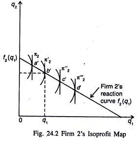
Iso-profit curves are lines showing those combinations of two competitors’ products q1 and q2 which yield a constant level of profit to firm 2. Profits of firm 2 will increase as it moves to iso-profit curves what are further and further to the left.
ADVERTISEMENTS:
This is so because if firm 2 fixes its output at some level, its profits will increase as firm 1’s output falls. Firm 2 will make the maximum amount of profit when it is a monopolist, i.e., when firm 1 decides to produce zero unit of output. In such a situation the Cournot model will generate sub-optimal outcome. Otherwise the model’s outcome is optimal since Cournot equilibrium is equivalent to the Nash equilibrium of games. And it is a model of symmetric oligopoly.
For each possible level of firm 1’s output, firm 2 wants to choose its own output in order to make its profits as large as possible. This means that for each level of firm 1’s output (q1), firm 2 will choose the level of output (q2) that put it on the iso-profit curve farthest to the left as illustrated in Fig. 24.2.
Reaction Curves:
At the optimum points the slope of each iso-profit curve must be infinite. The locus of these tangency points is firm 2’s reaction curve, f2(q1).The reaction curve gives the profit-maximising output of firm 2, for each level of output of firm 1. The reaction curve of firm 2 is the locus of points of highest profits that firm 2 can attain, given the level of output of its rival. It is called the ‘reaction curve’ or the best response curve because it shows how firm 2 will determine its output as a reaction to firm 1 ‘s decision to produce a certain level of output.
Firm 1’s reaction curve is shown in Fig. 24.1. Its output is a function of firm’s 2 output level so q1 = f1 (q2) just as q2 = f2(q1). Each reaction curve shows the relationship between a firm’s profit-maximising output and the amount it thinks its competitor will produce.
ADVERTISEMENTS:
Firm 1’s profit- maximising output is thus a decreasing function of how much it thinks firm 2 will produce. For each choice of output by firm 1 (q1), firm 2 chooses the output level q2 = f2(q1) associated with the iso-profit curve farthest to the left. At the optimum point the slope of each iso-profit curve of firm 1 is zero. Similarly for firm 2, it is infinite. In this model there is zero conjectural variation.
Cournot Equilibrium:
Each firm’s reaction curve tells us how much to produce, given the output of its competitor. In equilibrium, each firm sets output according to its own reaction curve. The equilibrium output levels are, therefore, found at the intersection of the two reaction curves in Fig. 24.3 (point E). We call the resulting set of output levels Cournot equilibrium.
Cournot’s equilibrium (which indicates how much output will each firm produce) is determined by the intersection of the two reaction curves (point E). At such a point, each firm is producing its profit-maximising level of output given the output choice of the other firm. In this equilibrium, each firm correctly assumes how much its competitor will produce and it maximises its profit accordingly.
Stability:
The Cournot equilibrium is a stable one, provided firm l’s reaction curve is that of firm 2. In Fig. 24.3 we start with output (q1t, q2t) which are not equilibrium outputs. Given firm 2’s level of output, firm 1 optimally chooses to produce q1t + 1 its next period. This point is located by moving horizontally from point A to the left until we hit firm 1’s reaction curve at point E.

If firm 2 expects firm 1 to continue to produce q1t+1 its optimal response is to produce q2t+1 at point B. Now firm 1 produces q1t+1 firm 2 will react by producing q2t+1. We find this point C by moving vertically upward until we hit firm 2’s reaction curve. The direction of arrows indicates the sequence of output choices of the two firms. Through such movements in a the ‘stair step fashion’, we trace out an adjustment process which converges to the Cournot equilibrium point (E). Thus Cournot equilibrium is stable.
Criticisms of the Cournot Model:
Let us suppose the two firms are initially producing output levels that differ from the Cournot equilibrium. The Cournot model does not say anything about the dynamics of the adjustment process, i.e., whether the firms adjust their output until the Cournot equilibrium is reached.
In truth, during any adjustment process, the central assumption of the model (i.e., each firm can assume that its competitor’s output remains fixed) will not hold. Since both firms would be adjusting their outputs, neither output would remain fixed. Such dynamic adjustment is explained by other models.
Cournot’s adjustment process is somewhat unrealistic. Each firm is assuming that the other’s output will remain fixed from one period to the next, but both firms keep changing their output levels. It is rational for each firm to assume that its competitor’s output remains fixed only when the two firms are choosing their output levels only once because then their output levels cannot be changed. It is also rational, once they are in Cournot equilibrium, for neither firm to change its own output.
The basic assumption about the behaviour of the two firms in the Cournot model is unrealistic. Each duopolist acts as if his rival’s output were fixed. However, this is not the case. If equilibrium is supposed to be reached through a sequence of finite adjustments, only one duopolist sets an output to start with; this induces the other to adjust its output which, in turn, induces the first firm to adjust its output once again, and the process goals so on and on.
It is quite unlikely that each will assume that his quantity decisions do not affect that of his rivals if each of his adjustments is immediately followed by a reaction on the part of his rival. If equilibrium is assumed to be reached simultaneously, the optimal quantity of duopolist 1 is not given by q1 = f1(q1), but by q1 = f1(q2), and similarly for 2, since each knows the behaviour pattern of the other.
Alternatively, it has been assumed that each maximises his profit on the assumption that his rival’s price remains unchanged. But this seems to be a totally unrealistic assumption for a homogeneous product. Duopolists and oligopolists generally recognise their mutual interdependence.
Only in equilibrium is one firm’s expectation about the other firm’s output choice actually fulfilled. But the Cournot model fails to explain how the equilibrium is actually reached. It can be used to focus only on the issue of how the firms behave in the equilibrium situation. Thus when using the Cournot model, we must, therefore, confine ourselves to the behaviour of firms in equilibrium.
Extension of the Cournot Model: The Case of Many Firms:
It is possible to generalize the Cournot model by considering a situation in which there are many firms. Here we assume that each firm has an expectation about the output choices of the other firms.
Let us suppose there are n firms and industry output Q is the joint contribution of all the firms, i.e., Q = q1 + q2 + … qn.
For an industry with V firms, the total equilibrium output for a Cournot oligopoly is given by Qn = Qc (n/n+1) where n > 1 and Qc is the output resulting from a perfectly competitive market.
Then the profit-maximising condition for firm i is:
Here the ten, e (Q)/si is the elasticity of the demand curve faced by the firm: the smaller the market share of the firm, the more elastic the demand curve it faces. In an extreme situation in which si = 1, the firm is a monopolist. In this case the demand curve facing the firm is the market demand curve. So the equilibrium condition is the same as that of a monopolist, i.e., MR = MC, where MR = p(Q) [1 – 1/|e(Q)|].
If in another extreme situation, the firm is a very small part of a large market, its market sharers virtually zero, and the demand curve facing the firm is completely elastic, in which case p = MC as is the case with a firm under pure competition. Thus if there are a large number of firms, none can exert much influence on the market price. In this case, the Cournot equilibrium is very similar to competitive equilibrium.
An Alternative Approach:
The Cournot model is a one-period method in which each firm has to forecast the other firm’s output choice. The two firms are assumed to produce a homogeneous product. The basic behavioural assumption of the model is that each duopolist maximises his profit on the assumption that the quantity produced by his rival is invariant with respect to his own quantity decision. Firm 1 maximises π1 with respect to q1, treating q2 as a parameter and firm 2 maximising π2 with respect to q2, treating q1 as a parameter.
Let us assume, to start with, that firm 1 expects that firm 2 will produce q2e units of output, where e stands for expected output. If firm 1 decides to produce q1 units of output, it expects that the total output produced will be Q = q1 + q2e and industry output will yield a market price of p (Q) = p (q1 + q2e).
The profit-maximisation problem of firm 1 is then:
max π1 = p(q1 + q2e) q1 – c(q1)
For any given belief about the output level of firm 2, q2e there will be some optimal choice of output for firm 1, q1.
This functional relation between the expected output of firm 2 and the optimal output choice of firm 1 can be expressed as:
q1 = f1(q2e)
This functional relation is simply the reaction function, which gives firm 1’s optimal choice as a function of its beliefs about the firm 2’s choice.
Similarly, we can derive firm 2’s reaction curve as:
q1 = f1 (q2e).
which gives firm 2’s optimal choice of output for a given expectation about firm 1’s output, q1e.
In the Cournot model each firm chooses its output level assuming1 that the other firm’s output will be q1e or q2e. Now we have to find out an output combination (q1*, q2*) such that the optimal output level for firm 1, assuming that firm 2 produces q1* is q2*is and the optimal output level for firm 2, assuming that firm 1 stays at q1* is q2*.
In other words, the output choices1 (q1*, q2*) satisfy:
q*1 = f1(q*2), q*2 = f2(q*1).
Such a combination of output level is known as a Cournot equilibrium. In a Cournot equilibrium, each firm is maximising its profits, given its beliefs about the other firm’s output choice. Moreover these beliefs get confirmed in equilibrium, with each firm optimally choosing to produce the amount of output that the other firm expects it to produce.
We know that in the Cournot model each firm has to forecast the other firm’s output choice. Given its forecast, each firm then chooses a profit-maximising output for itself. So the Cournot model seeks an equilibrium in forecasts — a situation where each firm finds its beliefs about the other firm to be confirmed. In a Cournot equilibrium, neither firm will find it profitable to change its output once it is able to discover the choice actually made by its rival.
Comments are closed.