
ADVERTISEMENTS:
The following points highlight the top two models of trade cycle. The models are: 1. Samuelson’s Model of Business Cycle 2. Kaldor’s Model of the Trade Cycle.
1. Samuelson’s Model of Business Cycle:
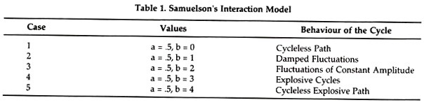
Prof. Samuelson constructed a multiplier-accelerator model assuming one period kg and different values for the MPC (a) and the accelerator (b) that result in changes in the level of income pertaining to five different types of fluctuations. The Samuelson model is
Yt= Gt +Ct+ It … (1)
ADVERTISEMENTS:
where Y is national income Y at time t which is the sum of government expenditure Gt, consumption expenditure Ct and induced investment It.

According to Samuelson, “If we know the national income for two periods, the national income for the following period can be simply derived by taking a weighted sum. The weights depend, of course, upon the values chosen for the marginal propensity to consume and for the relation (i.e. accelerator)”. Assuming the value of the marginal propensity to consume to be greater than zero and less than one (0< a <1) and of the accelerator greater than zero (b > 0), Samuelson explains five types of cyclical fluctuations which are summarised in the Table 1.
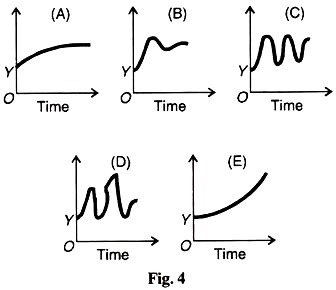
Case 1 – Samuelson’s case 1 shows a cycle less path because it is based only on the multiplier effect, the accelerator playing no part in it. This is shown in Fig. 4 (A).
ADVERTISEMENTS:
Case 2- shows a damped cyclical path fluctuating around the static multiplier level and gradually subsiding to that level, as shown in Fig. 4 (B).
Case 3- depicts cycles of constant amplitude repeating themselves around the multiplier level. This case is depicted in Fig. 4 (C).
Case 4- reveals anti-damped or explosive cycles, see Fig. 4 (D).
ADVERTISEMENTS:
Case 5- relates to a cycle less explosive upward path eventually approaching a compound interest rate of growth, as shown in Fig. 4 (E).
Of the five cases explained above, only three cases 2, 3 and 4 are cyclical in nature. But they can be reduced to two because case 3 pertaining to cycles of constant amplitude has not been experienced. So far as case 2 of damped cycles is concerned these cycles have been occurring irregularly in a milder form over last half century.
Generally, cycles in the post-World War II period have been relatively damped compared to those in the inter-World War II period. They are the result of “such disturbances—which may be called erratic shocks—arising from exogenous factors, such as wars, changes in crops, inventions and so on ‘which’ might be expected to come along with fair persistence.” But it is not possible to measure their magnitude.
Case 4 of explosive cycles has not been found in the past, its absence being the result of endogenous economic factors that limit the swings. Hicks has, however, built a model of the trade cycle assuming values that would make for explosive cycles kept in check by ceilings and floors.
Critical Appraisal of the Model:
The interaction of the multiplier and the accelerator has the merit of raising national income at a much faster rate than by either the multiplier or the accelerator alone. It serves as a useful tool not only for explaining business cycles but also as a guide to stabilisation policy.
As pointed out by Prof. Kurihara, “It is in conjunction with the multiplier analysis based on the concept of marginal propensity to consume (being less than one) that the acceleration principle serves as a useful tool of business cycle analysis and a helpful guide to business cycle policy.”
The multiplier and the accelerator combined together produce cyclical fluctuations. The greater the value of the accelerator (b), the greater is the chance of an explosive cycle. The greater the value of the multiplier, the greater the chance of a cycle less path.
ADVERTISEMENTS:
Limitations:
Despite these apparent uses of the multiplier-accelerator interaction, this analysis has its limitations:
(1) Samuelson is silent about the length of the period in the different cycles explained by him.
(2) This model assumes that the marginal propensity to consume (a) and the accelerator (b) are constants, but in reality they change with the level of income so that this is applicable only to the study of small fluctuations.
(3) The cycles explained in this model oscillate about a stationary level in a trendless economy. This is not realistic because an economy is not trendless but it is in a process of growth. This has led Hicks to formulate his theory of the trade cycle in a growing economy.
(4) According to Duesenberry, it presents a mechanical explanation of the trade cycle because it is based on the multiplier-accelerator interaction in rigid form.
(5) It ignores the effects of monetary changes upon business cycles.
2. Kaldor’s Model of the Trade Cycle:
Nicholas Kaldor built a model of the trade cycle based on the Keynesian terminology of saving and investment. He showed that the cycle is the result of pressures that push the economy toward the equality of ex-ante (anticipated, expected or planned) saving and investment. In fact, it is the difference between ex-ante saving and investment that leads to a cycle.
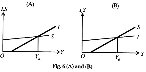
Kaldor shows the stability and instability conditions in the form of linear diagrams, though the cycle is only possible when I and S are non-linear. Take Figure 6 (A) and (B) where I and S are equal at the equilibrium level of income Y0. But in each case there is a single equilibrium position. In Panel (A) of the figure where I>S there is an unstable equilibrium position beyond Y0 because such a situation will lead to limitless expansion, to full employment and hyper-inflation.
On the other hand, if S>I, it means a downward movement to the left of Y0 which will lead to zero output and employment and to collapse of the economy as shown in Panel (B) of the figure. Kaldor discards linear saving and investment functions because they fail to produce a cycle. Instead, be adopts non-linear saving and investment functions.
A non-linear investment function I is shown in Figure 7. As the economy moves into the expansion phase, shown by the movement from the left along the I curve, the curve is almost flat. It means that there is excess capacity at a low level of income and the net investment is zero. But “when expansion gets under way, the negative effect of accumulated capital is a more powerful influence for investment decisions than the higher levels of output and profit.

In the opposite case of a high level of income when the economy moves into the contraction phase, the I curve is again flat and the net investment is small “because rising costs of construction, increasing costs and increasing difficulty of borrowing will dissuade entrepreneurs from expanding still faster.”
This slows down the rate of increase in output. It means that the existing capital stock and the capacity are more than the current output. This leads to decline in further investment. Thus income falls and the cumulative effect is that the economy moves into the contraction phase.
Similarly, a non-linear saving function is shown in Figure 8. At very low levels of income, saving is much reduced and may even be negative. So during the expansion phase, the MPS is large. At normal levels of income, saving will increase at a smaller rate. This is shown by the middle range of the S curve. But at very high income levels, saving will be absolutely large and people will save a large proportion of their income.

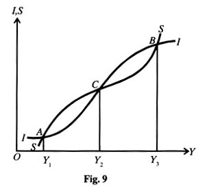
The cycle is visible when the non-Linear saving and investment curves are brought together, as in Figure 14. The figure shows multiple equilibria at positions A, B and C. Of these, A and B are stable positions and C an unstable position. Between positions C and B and below position A, I is greater than S. This will lead to the rise in income level. Between positions A and C and above B position, S is greater than I. This will lead to the fall in income.
But A and B are stable positions only in the short run. It is only in the long run that they become unstable and the path of the cycle is visible. For this, Kaldor introduces the capital stock as another variable that affects the relationship between saving and investment.
He takes both saving and investment as functions of income and capital stock so that S = f (Y, K) I = f (Y, K) and ds/dY> 0, ds/dK >0dI/dY> 0,dI/dK<0 and dI/dY> dS/dY, that is MPI is greater than MPS over the expansion or contraction phase of the cycle.
The above relationships show that both S and I vary positively with Y; while S varies directly with K, and I varies inversely with K. The relationship MPI > MPS shows the instability of the economy which will move it either toward expansion or contraction.
In terms of Figure 9, positions A and B are “switch points” in the long run. They are the points at which the economy alters its direction either toward expansion or contraction. Point C is unstable in both directions. It is only when points C and B come closer, the expansion phase of the cycle starts. When they are joined, expansion stops and contraction begins. On the contrary, when C and A come closer contraction starts. When they are joined, contraction stops and expansion begins.
Expansion Phase:
Kaldor shows the expansion phase of his trade cycle in three stages, as shown in Figure 10. Starting from position Y0 in figure stage 1 (which is the same as Figure 8), suppose the economy is in equilibrium at point C. But this is the point of unstable equilibrium. An upward displacement shows that I>S which leads to the economy towards the expansion path.
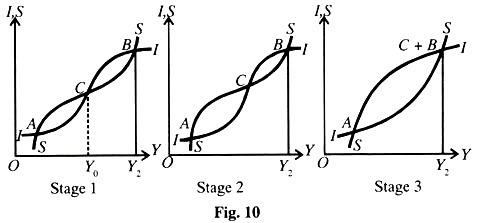
As the rate of investment is high, the economy’s capital stock increases at a rapid rate. But as the capital stock increases, the MEC declines and investment curve shifts downward At the same time as the economy’s capital stock increases, it raises the income of the economy thereby raising its saving. Thus the saving curve shifts upward. So a downward shift of the investment curve I and upward shift of the saving curve S bring the point C nearer to B, as shown in figure stage 2.
This process of the downward shifting of the I curve and upward shifting of the S curve continues till the two curves are tangential and points C and B coincide, as shown in figure stage 3. But at this position S>I in both directions. So this is an unstable equilibrium position in the downward direction. This leads to the downward movement of the economy till point A is reached in stage 3.
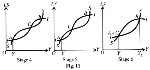
Contraction Phase:
The contraction of the trade cycle is also shown in three stages, as in Figure 16. We start from position Y1 corresponding to point A in stage 4 of the figure. It is the point of short-run stable equilibrium but at a very low income level. But over the long run at such a low level of income, the capital stock decreases due to excess capacity and the investment curve I shifts upward. Simultaneously, saving falls which shifts the saving curve downward.
Thus the shifting of the I curve upward and of the S curve downward bring positions A and C nearer, as shown in stage 5. This process will continue gradually till I and S curves arc tangential and positions A and C coincide, as in stage 6 figure. But this A+C position at Y, income level is unstable in the upward direction because I>S. This will lead to an expansionary process till the economy reaches the higher level of income Y2 at point B. From B, the I and S curves gradually reach the positions shown in stage 1 of Figure 11, and again the cyclical process starts. Thus Kaldor’s cyclical process is self-generating.
According to Kaldor, the forces which bring about the lower turning point are not so certain at the higher level. “A boom left to itself, is certain to come to an end; but the depression might get into a position of stationariness, and remain there until external changes (the discovery of new inventions or of the opening up of new markets) come to the rescue.”
Further, cycles in the Kaldor model are not necessarily of the same length and duration. Neither are expansions and contractions necessarily symmetrical. In fact, these depend upon the slopes of the I and S curves and the rate at which they shift in each phase of the cycle.
Kaldor neither uses the acceleration principle nor the monetary factors in explaining his theory of the trade cycle. At the same time, he demonstrates how a cycle could exist in the absence of any growth factor.
Comments are closed.